Open Problems solved by Frontier AI
Over the last year, and a better part of this year, a number of open problems have been solved by Frontier AI models. In this post, I have handpicked a few problems :- Erdos’s Unit distance problem, Claude Cycles (an open problem by Donald Knuth), Cosmic String Spectra Integral and the recently disproven Jacobian conjecture (counter-example).

Table of contents
- Introduction
- Erdos Unit Distance Problem
- Claude Cycles
- Cosmic String Spectra
- The Jacobian Conjecture - (CounterExample)
- Conclusion
- Cite this work
Introduction
The last few years , especially since the scaling era began (post GPT-2 release), has been fascinating to say the least for open problems. Beginning in 2021, with AlphaFold, the potential for frontier models to solve open problems across disciplines has been a central point of discussion in the scientific community. AlphaFold, which was developed by DeepMind , had predicted 3D co-ordinates for all heavy atoms for a given protein using the primary 1D amino acid sequence, thus solving the “protein-folding” problem. It predicted the structures with near experimental accuracy and this extraordinary feat earned Demis Hassabis and John Jumper from Google DeepMind, the Nobel Prize in Chemistry in 2024.
The inflection point which I believe was in 2024, when once again, AlphaProof of Google DeepMind’s combined AlphaProof and AlphaGeometry 2 systems achieved the silver-medal standard, solving four out of the six highly unseen , original math contest problems. AlphaProof had utilized Deep-RL(similar to AlphaZero) for the proof. In November 2025, it was announced that Harmonic’s Aristotle had solved a simplified variant of the Erdos problem #124.
I wasn’t really planning on writing about this, but over the last year and the better part of this year , a number of open problems have been solved by Frontier models. This has sparked a curious investigation among researchers as well as the lifelong critics who were quick to dismiss LLM capabilities as nothing more than “stochastic parrots”. Further verification is still going on to find complete solutions as I am writing this piece.
As for my own personal opinion, I think this is an excellent time for us to define what truly constitutes as “intelligence” as more open problems continue to be solved.
Since my time nowadays is almost equally divided between AI and theoretical physics, I thought it would be a fairly decent exercise if we went through some of the problems to understand AI’s contribution in detail. I have picked a few problems for this specific post. Let’s get into these.
FunSearch
In late 2023, DeepMind had introduced FunSearch (short for searching in the function space)- an evolutionary procedure that is based on pairing a pre-trained LLM with a systematic evaluator. The paper focuses on problems that rely on an efficient evaluate function, which measures the quality of a candidate solution. The goal with FunSearch was to generate a solve program, such that it’s outputs receive high scores from eval (when executed on inputs of interest ), and ultimately improve over the best known solutions. FunSearch had combined a pre-trained (frozen) LLM, whose goal was to provide solutions with an evaluator, which would then act as a guard against incorrect ideas. FunSearch iterates over these two components, evolving initial low-scoring programs into high-scoring ones , which discovers new knowledge.
FunSearch addresses the Cap-Set Problem, which was an open challenge for decades. Terrance Tao had once described it as his favorite question. Upon collaborating with different authors, Funsearch generated solutions – which in some settings discovered the largest cap-sets ever found. Moreover, Funsearch had outperformed many other state of the art computational solvers.
Problem Statement:- The problem statement consists of finding the largest set of points (called a capset) in a high dimensional grid , where no three points lie on a line.
This is an important problem because it serves as a model for other problems in external combinatorics – the study of large or how small a collection of numbers, graphs or other subjects could be. Brute- force computing approaches to this problem usually do not work . The number of possibilities that are necessary to consider, quickly becomes greater than the number of atoms in the universe.
def priority(el: tuple[int, ...], n: int, w: int) -> float:
	score = 0.0
	for i, el_i in enumerate(el):
		if el_i == 1:
			score -= 0.2 ** (i * 0.5)
		if el_i == 0:
			score -= 0.3
		else:
			score -= 0.7 ** i
	return score
The above is the code generated by FunSearch yielded further actionable insights
These results demonstrate that the FunSearch technique can take us beyond established results on hard combinatorial problems, where intuition can be difficult to build.
One thing that is important to note here is that, these problems weren’t solved in isolation, meaning there were always humans in the loop. A prompt was provided, on the basis of which the models took appropriate steps. This isn’t to say that humans weren’t there to check rigorously . The solution provided by these models were then independently verified by researchers.
Erdos Unit Distance Problem
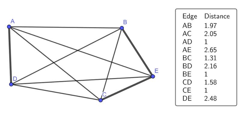
Figure:-1:- Unit Distance Problem.(credit:- ARStechnica)
In 1946, Paul Erdos had proposed a deceptively simple question in discrete geometry:
Problem Statement:- Given $n$ points in the plane, what is the maximum possible number of pairs of points that are exactly $1$ unit apart ?
Suppose you have $5$ points in the plane. Some pairs of them may happen to sit at a distance of exactly $1$ from each other. The question is:- how many such unit distance pairs can one maximally create by cleverly arranging $n$-points ?. As $n$ grows large, finding the exact answer becomes extraordinarily difficult, so instead Erdos had focused on finding the Upper and Lower bounds - i.e, how fast does this maximum number grow as a function of $n$ ?.
- Lower Bound:- Erdos had observed that, if you placed points in a square grid, with carefully chosen spacing, many pairs will be exactly one unit apart. The trick relies on the Pythagorean theorem: if a point is $a$ units right and $b$ units up from another, the distance is $\sqrt{( a^2 + b^2)}$. by choosing grid spacing so that $a^2 + b^2 = 1$ for many integer pairs $(a, b)$, each point can be unit distance from many neighbors. For example:- Suppose $a^2 + b^2 = c^2$, the trick is to choose some number $c^2$ so that there are a whole bunch of pairs of whole numbers $a$ and $b$ such that $a^2 + b^2 = c^2$. Then, if we can scale the grid down so that each point is $\frac{1}{c}$ from its neighbors, there will be a bunch of unit distances. For eg:- if we choose, $c^2 = 25$, then the Pythagorean theorem can be satisfied by either $0^2 + 5^2 = 25$ or $3^2 + 4^2 = 25$. This corresponds to a $12$-grid point circle with points $(0,5), (3,4), (4,3), (-4, 3),(-3, 4),….$ etc. In short, we want to choose a $c^2$ that is large enough, but not too large. Using insights from number theory, including Jacobi’s two-square theorem, Erdos was able to show that an optimally sized circle will enable the number of unit-distance pairs to grow faster than the number of points but barely. So, the previous best construction that was shown by Erdos, came from a rescaled squared grid that yielded roughly $n ^ {(1 + \frac{C}{\log \log n})}$ unit distances – that was barely faster than linear growth. $C$ was a constant. Since $\log \log (n)$ tends to infinity with $n$, the additional terms in the exponent tends to $0$. Thus slightly faster than traditional growth. For decades, it was believed that it was the best rate which was possible , and no construction could significantly improve over the square grid.
- Upper Bound:- The best known lower bound had largely remained unchanged since Erdos’s original 1946 construction. The best upper bound $O(n^{\frac{4}{3}})$ , dates to the work of Spencer and Trotter in 1984, and remained unchanged. Erdos had conjectured that the true maximum was much closer to his lower bound. In other words, Erdos had believed that a square grid was essentially optimal , and one couldn’t do dramatically better, no matter how cleverly the points were arranged. He conjectured that an upper bound of $n^{(1 + O(1))}$, meaning that for a large $n$, it (the maximum number of distances) grows slower than $n^{(1 + \epsilon)}$ for any $\epsilon > 0$. For 80 years, this conjecture had stood. Most mathematicians had believed that Erdos was right. However, they were unable to prove it and the tools to do so seemed nowhere near as close.
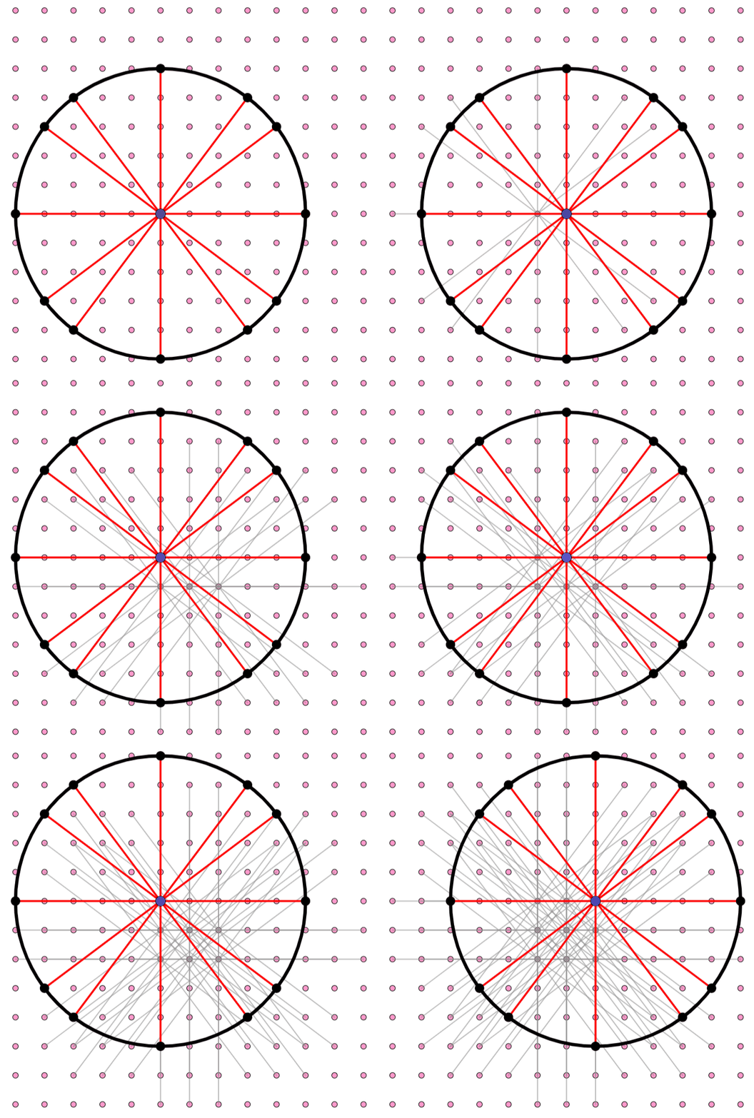
Figure 2:- An animation of the distance-one neighbors of nine central points in a 13×13 grid. You can draw similar circles for other points in the grid to get the remaining distance-one pairs, but some points on the circle won’t land on grid points. Credit: Kai Williams / Understanding AI
The question therefore became – can we do better ?
On May 2026, OpenAI announced that one of it’s internal reasoning models had disproved Erdos’s Conjecture. This was the first time an AI system had autonomously produced a proof resolving a major open mathematical conjecture. It didn’t prove Erdos right. It actually, proved him wrong..!!.
For infinitely many values of $n$, the proof constructs configuration of $n$ points with at least $n^{(1 + \delta)}$ unit distance pairs, for some fixed $\delta > 0$ . Professor Will Sawin has shown that one can take $\delta = 0.014$.
The model had constructed a grid in a high dimensional space and then projected this more complex structure into two dimensions. And instead of using a whole-number grid with points like $(1,3)$ or $(-3, 6)$, the model had used something called algebraic integers to build this more complicated grid. It turns out that this kind of high-dimensional grid has richer structure which allows the AI to pack more unit distances in the same number of points original disproof.
The key breakthrough was applying tools from
algebraic number theory (Golod - Shafarevich theory) to
discover infinite family of patterns. This theory was applied to a combinatorial geometry problem. The solution
required grinding through many processes that seemed unlikely to succeed. University of
Toronto professor (he won the fields medal as I was writing this piece) Jacob Tsimerman noted
that he had briefly considered a similar approach but abandoned
it because “it consumes too much time and frequently does not work out”.– he had mentioned this
in an OpenAI document. While the model’s proof does not provide an explicit formula, mathematician
Will Sawin (who was part of the verification effort) extracted from it that the number
of unit distances grows at least at the rate of $n · exp(C·√(\log n))$ – which for
a large $n$ becomes much larger than $n ^ {(1 + \frac{C}{\log \log n})}$. This decisively
breaks Erdos’s $n^{(1 + O(1))}$ upper bound. The result has since been verified by multiple
mathematicians and the proof was posted here
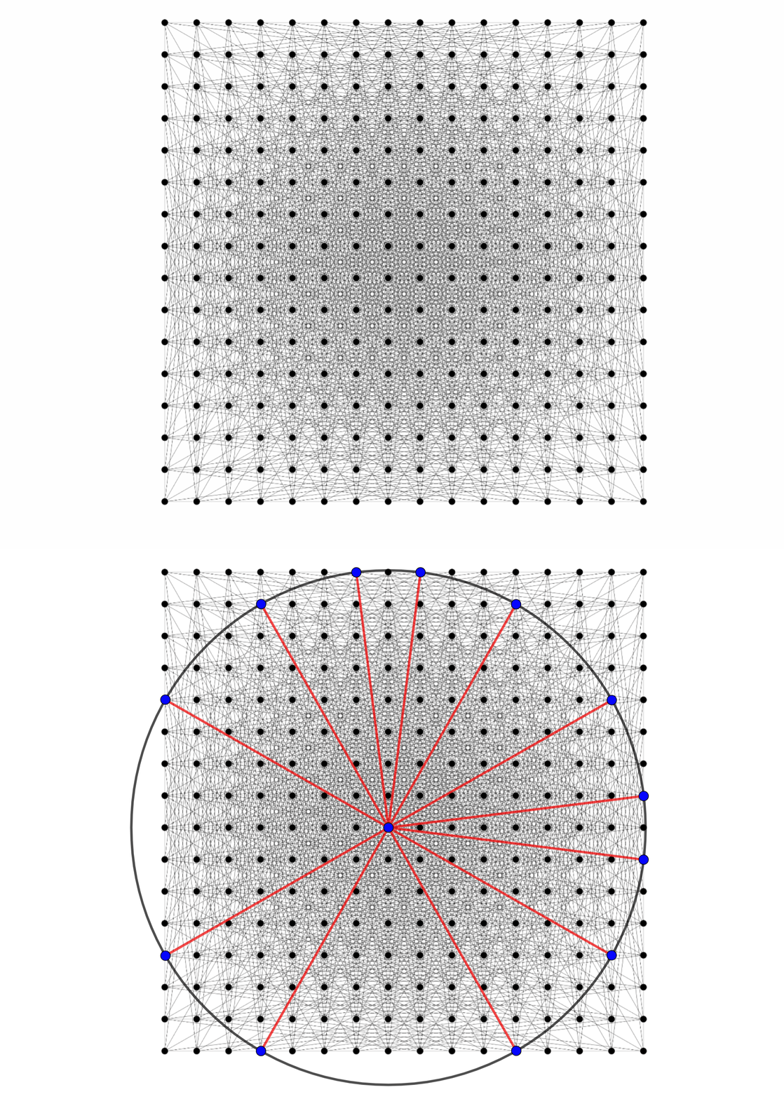
Figure 3:- A diagram from OpenAI’s announcement of the AI’s disproof of the unit distance conjecture, onto which I superimposed a circle showing the distance-one neighbors for one point. The grid spacing here is 1/√65, which produces unit circles that intersect 16 points on the grid (or would if the grid were larger). Credit: Kai Williams / Understanding AI
Why does this matter
The reason why this matters is because it is one of the first known conjectures to be autonomously disproved. Field’s medalist Terrance Tao had called it “A milestone in AI mathematics”. Later on in the post , we are going to encounter another one of these conjectures which has been disproven by Claude’s fable 5. Another reason which I think is essential to be understood is that it didn’t just brute-force a problem, it used existing methods like algebraic number theory to discover an entirely new family of geometric constructions. As ARS- Technica- One of the sources I have used to study about Erdos’s Unit distance conjecture has aptly put - “ more in line with past AI efforts than the headline result might suggest.”. While the AI found the proof autonomously, humans verified it, refined it, and extended it (e.g., Sawin’s explicit lower bound).
It is important to note that the problem is yet to be fully resolved. The best known upper bound still remains around $n^{(\frac{4}{3})}$ , leaving a significant gap for the upper and lower bounds. But Erdos’s original conjecture – that the answer was just barely above linear, has now been definitively proven to be false.
For one thing, other companies have also worked to solve Erdős problems. Because Erdős posed hundreds of problems over his career—and because mathematician Thomas Bloom has organized an effort to compile all of them at www.erdosproblems.com—AI companies have used them as a testing ground to evaluate AI systems. In January, Cambridge undergraduate Kevin Barreto worked with a friend to ask GPT-5.2 and the aforementioned Harmonic’s Aristotle to produce the first autonomous solution of an Erdős problem. On May 22, two days after OpenAI’s announcement, Google announced that its AI system had solved nine open Erdős problems, including two that had been open for over 50 years.
You can click here if you want to play with the illustration yourself.
Moving on, another problem that I want to discuss was an open problem by Donald Knuth
Claude Cycles
“Shock ! Shock !” is what Donald Knuth- one of the living legends in computer science , opens his paper with. Upon learning that Claude Opus 4.6 had successfully solved a problem he had been working on for weeks, Knuth exclaimed that he needed to revise his opinions on “generative AI” and it’s ability to solve open problems. But before getting into the crux of the problem that Knuth was stuck on for weeks , a few fundamental terms and definitions from Graph Theory are in order.
- Digraph:- In graph theory, a digraph is a set of vertices (nodes) connected by edges , where the edges have a specific direction. Formally speaking, a digraph is denoted as $G = (V, A)$ , where $V$ is the set of vertices and $A$ is the set of directed arcs. An arc here from vertex $u$ to vertex $v$ is written as $(u, v)$.
- Degrees:- In a digraph, each vertex has two distinct degree measures . In degree:- The number of incoming edges to a vertex and Out Degree:- The number of outgoing edges from a vertex.
- Paths and Cycles:- A path follows the direction of the arrows. A directed cycle occurs when a sequence of edges begins and ends at the exact same vertex, moving only in the direction of arrows.
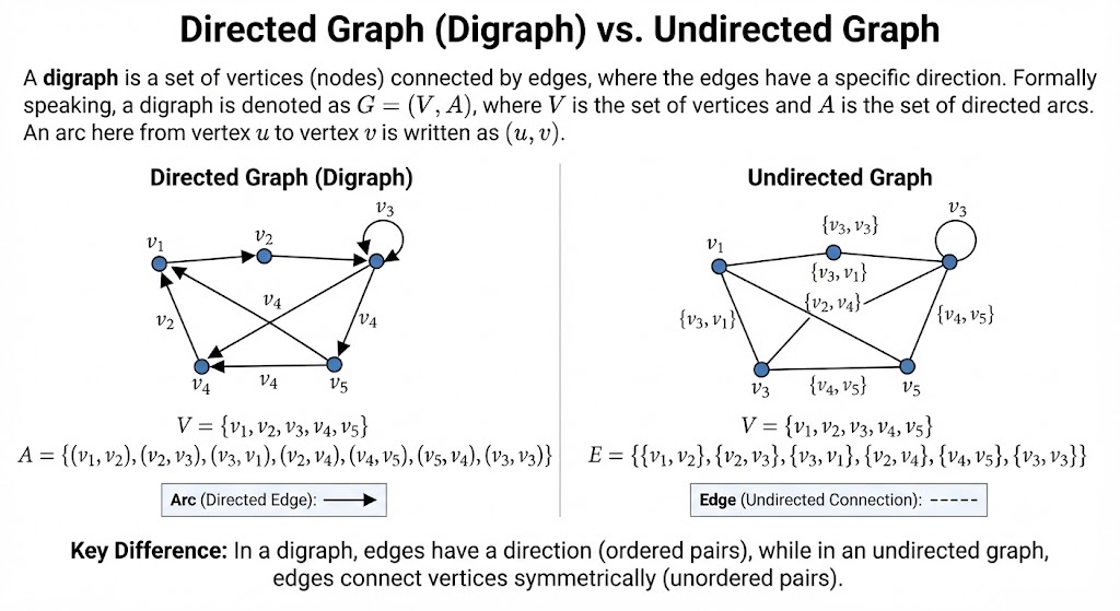
Figure 4:- Directed vs Undirected Graph
Now imagine a $3D$ grid of points like for example:- a Rubik’s Cube. Specifically, a Rubik’s cube that is made up of tiny dots. Say, you have $5$ dots along each edge giving you $5 \times 5\times 5 = 125$ dots total. Now, in a normal grid, the dots on the edges and corners have fewer neighbors. But, on a torus, the edges wrap around. Like, for instance in a game like Pac-Man, where walking off the right-side of a screen , brings you back on the left. In $3D$ , wrapping happens in all three directions. So, every single dot has exactly $3$ neighbors that it can move to:-
- One-step in the $x$- direction.
- One-step in the $y$- direction.
- One-step in the $z$- direction.
So, in a digraph, from each dot there are exactly 3 arrows that are pointing outward to its three-neighbors. That is the whole structure:- dots arranged in a $3D$ wrapping grid , with one-way arrows along each axis.
- Hamiltonian Cycle:- A Hamiltonian Cycle is simply a tour, that visits every single dot exactly once and returns to where you had started following the arrows. You can think of it as a delivery route , we need to visit every house in the neighborhood (every dot), you can only travel along the allowed one-way streets ( the arrows) , you cannot visit any house twice and you must end up back home.
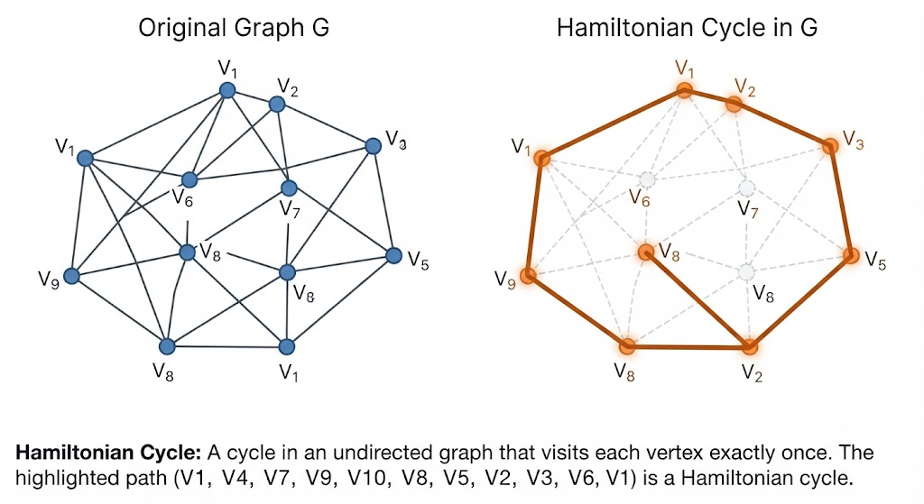
Figure 5:- Example of a Hamiltonian cycle
The tricky part here is that the torus digraph with $m^3$ dots ( eg:- $125$ dots), you need a single unbroken loop of exactly $125$ arrows that hit every dot. With so many dots and so few choices at each step (only $3$ arrows) , it is surprisingly hard to find such a tour and even harder to find three of them that together use every arrow exactly once, which is what Knuth’s problem had asked for.
So, Donald Knuth had come up with a problem while writing about Hamiltonian cycles for a future volume of his book :- The Art of Computer Programming. The problem statement is as follows:-
Problem Statement:- Consider the digraph with $m^3$ vertices $i j k$ for $0 \le i, j, k < m$ and three arcs from each vertex, namely $i ^{+} j k$ , $ij^{+} k$ , $ijk^{+}$, where $i ^{+} = ( i + 1)$ mod $m$. Try to find a general decomposition of the arcs into three directed $m^3$ - cycles for all $m > 2$.
So, in somewhat simpler terms, his digraph can be laid out in $3D$ with the vertices at the integer co-ordinates. each point of the form $(i, j, k)$ is connected by a directed edge to three points , $(i + 1, j, k)$, $(i, j +1, k)$, $(i, j, k + 1)$.
These all lie within a cube of length $m$ on a side . A vertex at an edge is connected to a vertex at the other end in a wraparound. So given that Knuth is asking if we can find three different paths, each of which goes through all the vertices. In addition, each directed edge must be traversed exactly once by exactly one of the points blog
Now, according to the Claude cycles paper, Knuth had solved the problem for $n = 3$ and asked for the generalization as part of the answer. A friend of his Filip Stappers had empirically discovered solutions for $4 \le m \le 16$ .
What Claude Proved
So after $31$ explorations: At first it had reformulated the problem. It had assigned a permutation at each vertex and “each resulting functional digraph must be a single Hamiltonian Cycle”. Then in its second attempt , it tried a DFS (Depth First Search) attempt. Thirdly it tried a $2D$ Serpentine analysis., simulated annealing and finally through pure mathematical reasoning, Opus 4.6 had produced an explicit construction that generates three Hamiltonian cycles decomposing the digraph for all odd $m > 1$. The construction uses a simple rule based on $S = ( i + j + k)$ mod $m$.
- When $S = 0$ , bump $i$ if $j = m -1$, otherwise bump $k$.
- When $0 \le S\le m -1$ , bump $k$ if $i = m-1$ , otherwise bump $j$.
- When $S = m -1$, bump $k$ , if $i = 0$, otherwise bump $k$.
Here, “bump” means “ increase by $1$ , mod $m$”. Strappers verified that this works for every odd $m$ from $3$ to $101$ . Knuth then provided a rigorous mathematical proof that it works for all odd $m$. Knuth then formalized what makes Claude’s construction work , proving a general theorem.
Theorem:- A Claude like decomposition (one where the permutation at each vertex depends only on whether each co-ordinate is $0$, $m-1$, or neither) is valid for all odd $m >1$, if and only if each of the three sequences that it defines is generalizable .
— meaning the $m = 3$ pattern lifts correctly to all larger odd $m$
Proof:- If those three sequences aren’t Hamiltonian , or they don’t generalize to Hamiltonian cycles for all odd $m > 1$, they certainly don’t define a valid decomposition. Conversely, if they are Hamiltonian cycles, they are definitely valid: Every vertex $i j k$ appears in each of the three cycles, and it’s three outgoing arcs are partitioned properly because $d$ is a permutation.
Here, decomposition is “Claude-like” if it can be generated by a C program like the one given in the paper, in which the permutations $d$ of $\{0, 1, 2 \}$ depend only on whether $i$, $j$, and $s$ are $0$ or $m−1$ or not. No special cases other than $0$ and $m−1$ are allowed to affect the choice of $d$. This is the assumption upon which, the theorem has been constructed.
Knuth shared that there are exactly 11,502 Hamiltonian cycles for $m=3$ . Of these, 1,012 generalize to $m=5$ , and 996 generalize to all odd $m>1$ (having passed the tests at $m=5$ and m=7 ). These 996 yield 4,554 valid decompositions of the $3 \times 3 \times 3$ digraph. Claude’s construction is one of these.
Now, so far we have been discussing about the odd case. For the even case, Claude found empirical solutions for $m = 4, 6, 8$ , but could not generalize. However, the paper’s breaking news addendum reports that:- GPT - 5.3 - codex had generated a decomposition for even $m \ge 8$ . Knuth had tested it for all even $m$ from $8$ to $200$ and also a bunch of random evens between $400$ to $2,000$ and according to him it “looks good”. GPT-5.4 (extended thinking) , then wrote a flawless 14 page construction, that the construction works for even values of $m$. Claude and GPT working together (via Keston Aquino-Michaels) produced an even simpler and valid decomposition for an odd $m$, together with an elegant decomposition for the case of even $m$.
Don Knuth , stuck on this problem for weeks , called it an “impressive success story”. Some of the key strengths that Claude had demonstrated was that : it had recognized th e digraph as a Cayley digraph and brought in methodologies from combinatorics and group theory. It sustained a multi-step reasoning after $31$ rounds of exploration and also escalated it’s strategies from time to time. It moved from simulated annealing (which “can find solutions but not give constructions”) to pure mathematical construction.
So, the reason why the problem was hard was because at every dot, you have 3 arrows going out, and one needs to assign each arrow to a different dot. But, if a wrong assignment is made anywhere , a route might get stuck on a short loop, visit a dot twice, or simply fail to reach all the dots. For a tiny $3 \times 3 \times 3$ grid (27 dots), one can brute-force it. But, Knuth needed a rule that could work for any size - $5 \times 5 \times 5$, $101 \times 101 \times 101$, a million dots without having to check for each case individually.
In simple terms, what Claude did was find a rule that tells you, for each dot, which arrow belongs to which route and this rule always works for grids of any odd size. No exceptions. Knuth then proved mathematically, that Claude’s decomposition construction is in fact correct. Simply speaking, Claude had discovered a universal recipe for splitting the arrows of any odd sized $3D$ wrapping grid into three perfect tour routes. “Shock! Shock !” is what Knuth begins the paper with. While initially it may seem that way, however, given what the capabilities of frontier models have displayed so far, solutions to open problems seem inevitable and Knuth concludes with “very interesting times indeed”. A considerable difference in optimism.
Shifting gears, we move into theoretical physics. A couple of interesting open problems has been solved in the last few months. One of them is the Cosmic Spectra Integral.
Cosmic String Spectra
Cosmic Strings can be considered as $1d$ topological defects, present in the early universe. When cosmic string networks intersect, they pinch off to form closed loops. These loops oscillate under immense tension, emitting energy primarily as gravitational waves. Cosmic string spectra typically refer to the unique signatures of gravitational waves emitted by oscillating loops of cosmic strings. Because these loops oscillate and decay over cosmic time, they produce a stochastic gravitational wave background and discrete, harmonic frequencies that differ from other astrophysical sources.
The thickness of a cosmic string is much smaller than any curvature scale of interest, whose dynamics are governed entirely by the geometry of it’s worldsheet - the two dimensional surface $X^\mu(\tau, \sigma)$ , traced out by the string as it evolves through spacetime. The action is the Nambu Goto action:- ( I am excluding the full derivation of a point-particle , worldvolume ). The action is given by:-
\[\begin{align} S_{NG} = -\mu \int d\tau d\sigma \sqrt{-det \gamma_{ab}} \end{align}\]where $\tau$ and $\sigma$ are the worldsheet co-ordinates (timelike and spacelike respectively) and $\gamma_{ab}$ is the induced metric on the worldsheet.
\[\begin{align} \gamma_{ab} = \eta_{\mu\nu} \partial_\alpha X^{\mu} \partial_{\beta} X^{\nu} \end{align}\]Here, $\eta_{\mu\nu} = diag(-1, +1, +1, +1)$ is the Minkowski metric and the indices run over $\{\tau, \sigma\}$ . The square-root of $-det \gamma_{ab}$ is the invariant area element of the worldsheet. The Nambu-Goto action is the direct analogue of the relativistic point particle action $-m \int d\tau \sqrt{(- \dot{x}^2)}$ , generalized from a worldline to a worldsheet. We are working in a conformal gauge where the induced metric is conformally flat (Assume that the temporal gauge has been fixed)
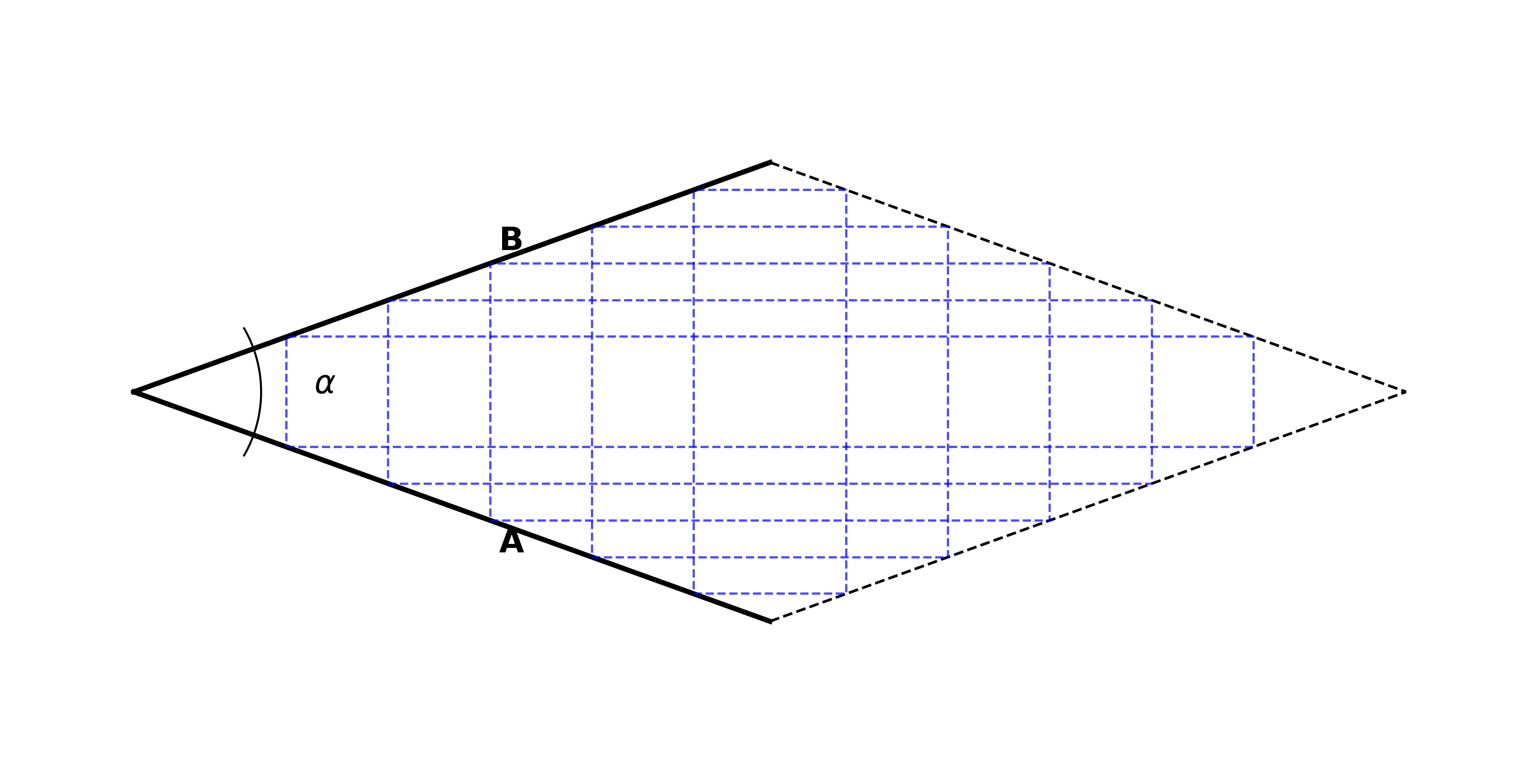
Figure 6:- Evolution of a GV loop with the indicated opening angle 𝛼. At any given time, the loop corresponds to one of the blue dashed rectangles:. Generated with the help of Kimi3. credit:- paper:
The Garfinkle-Vachaspati loops(GV Loops) , (paper, paper) , are a specific class of cosmic string loops that are modeled as planar, rectangular loops with 90 degree corners. (called kinks) , connecting four straight string segments. These loops are used to study how cosmic strings behave, radiate and evolve.
Some of the key characteristics of GV loops are as follows:-
- Unlike other string loops that form sharp, infinitely dense points called cusps, these loops only have sharp 90 degree corners.
- Because they lack cusps , they do not emit the sudden bursts of gravitational radiation seen in other loops. Instead, they decay smoothly by shredding energy over an entire lifetime.
As these strings vibrate, they emit gravitational waves. Researchers look at the “power spectrum” (the amount of energy released at different frequencies) to figure out what kind of waves, a string network might leave behind. Roughly speaking, there can be three plausible signature of this radiation. First the cusps on the string (moving near the speed of light) can emit strongly beamed gravitational radiation. Second, this gravitational radiation can produce a stochastic background. Thirdly, the pattern of radiation from a single oscillating cosmic string loop is sufficiently distinctive that it might be observable in future detectors. The power spectrum of gravitational radiation from cosmic strings is central to the calculation of the stochastic background which is produced in such models. The string network evolution has been provided in details in the above paper.
But, we are interested in the power spectrum $P_n$ of gravitational radiation which is produced by a given loop.
Cosmic string with cusps generally produce a power spectrum of the form $P_n \propto n^{-4/3}$ . The power spectrum $P_n$ is a quantity which is relevant for the stochastic background as a function of the $n$th harmonic. (A function of $n$ for the GV Loops) . Now, suppose we have a loop of length $L$ and at time $t$ , the power that is emitted at frequency $W_n = 4\pi n / L$ is given by,
\[\begin{align} \frac{dP_n}{d\Omega} = \frac{32 G\mu^2}{\pi^3 n^2} \end{align}\]Where $G$ is Newton’s gravitational constant, and $\Omega$ is the density per logarithmic frequency interval. $\mu$ is the string tension. The power spectrum $P_n$ is given by the core spectral integral over the unit sphere $S_2$ . Therefore, $P_n$ would be:-
\[\begin{align} P_n = \frac{32 G\mu^2}{\pi ^3 n^2} I(n, \alpha) \end{align}\]$I(n, \alpha)$ is calculated over the unit sphere. The factor $G\mu^2$ encodes the dimensionless coupling of the string to gravity, and the $1/n^2$ prefactor, reflects the generic fall-off of radiation power with harmonic number. $\alpha$ is the opening angle as was mentioned in the above figure 6. The entire dependence of the loop geometry (through $\alpha$) and the mode structure (through $n$) is captured by the single core spectral integral function $I(n, \alpha)$.
GV loop Solutions
Now, because we are working with closed string loops, we need periodic solutions for a loop of invariant length $L$ with periodicity $L/2$ in each mode, the left and right moving mode derivatives are:-
\[\begin{align} \mathbf{a}'(\sigma') = \hat{a}\,\cos\!\left(\frac{4\pi\sigma'}{L}\right), \qquad \mathbf{b}'(\sigma'') = \hat{b}\,\cos\!\left(\frac{4\pi\sigma''}{L}\right) \end{align}\]where $\hat{a}$ and $\hat{b}$ are {constant unit vectors} in $\mathbb{R}^3$ satisfying: $\hat{a} \cdot \hat{b} = \cos\alpha$ . The full trajectory is obtained by integrating the above equation . The $2D$ worldsheet $X^{\mu}(\sigma, t)$ traced out by the string is given by:-
\[\begin{align} \mathbf{X}(\sigma, t) = \frac{L}{4\pi}\left[\hat{a}\,\sin\!\left(\frac{4\pi(\sigma - t)}{L}\right) + \hat{b}\,\sin\!\left(\frac{4\pi(\sigma + t)}{L}\right)\right]\end{align}\]This closed-form expression of the string trajectory is the starting point for all subsequent radiation calculations. Now, in order to derive $I(n, \alpha)$ , one substitutes the GV- solution from the second equation into the wave-power formula. The stress energy tensor of a Nambu-Goto string is therefore :-
\[\begin{align} T^{\mu\nu}(x) = \mu \int d\tau\, d\sigma\; \dot{X}^\mu \dot{X}^\nu\; \frac{\delta^{(4)}(x - X(\tau,\sigma))}{\sqrt{-\gamma}}\end{align}\]The power emitted at harmonic $N$ involves a Fourier decomposition of $T^{\mu\nu}$. After performing the worldsheet integrals, the angular dependence can be isolated into an integral over the unit sphere $S^2$. The projection factors onto a generic direction $\hat{r}$ on the unit sphere. $e_1 = \hat{r} \cdot \hat{a}, \qquad e_2 = \hat{r} \cdot \hat{b}$.
The string oscillation modes contribute factors of the form $\bigl[1 - (-1)^n \cos(n\pi\, e_i)\bigr]$ arising from the Fourier decomposition of the string trajectory at harmonic $n$. The gravitational wave amplitude involves products of these factors (one from each mode) divided by the denominator factors $(1 - e_i^2)$. paper.The resulting integral is:
\[\begin{align} I(n, \alpha) = \int_{S^2} d\Omega\; \frac{\bigl[1 - (-1)^n \cos(n\pi\, e_1)\bigr] \bigl[1 - (-1)^n \cos(n\pi\, e_2)\bigr]} {(1 - e_1^2)(1 - e_2^2)} \end{align}\]The two unit vectors satisfy $\hat{a} \cdot \hat{b} = \cos\alpha$. The evaluation of this integral has been a long-standing open problem in theoretical physics.
Now, there are a few features that make the evaluation of this integral notoriously difficult to solve:-
- Singularities at the poles:- When $e_i \to \pm 1$ (i.e., when $\hat{r}$ aligns with $\hat{a}$ or $\hat{b}$), the denominator $(1 - e_i^2) \to 0$ while the numerator tends to $0$ as well, since $\cos(n\pi) = (-1)^n$. This is an indeterminate $0/0$ form — the integral is convergent by the vanishing of the numerator. But standard numerical rules fail catastrophically because finite-precision arithmetic cannot resolve the cancellation at the poles.
- High oscillation for large $n$:- As $n \to \infty$, the cosine terms start oscillating with frequency $\sim N\pi$ on the sphere. Direct numerical integration would require $O(n^2)$ . This prohibits for the high harmonics ($n \gg 1$) that carry the majority of the radiated power.
- Coupling between $\alpha$ and angular integration:- The angle $\alpha$ couples the two projection factors $e_1$ and $e_2$ through the dot product constraint $\hat{a} \cdot \hat{b} = \cos\alpha$, so the integral over $S^2$ does not factorize into two independent one-dimensional integrals. This non-separability is what makes the problem fundamentally two-dimensional and significantly harder than a single angular integral.
The first crucial step that the AI had also independently recognized, was to recast the core spectral integral by defining,
\[\begin{align} f_n(t) = \frac{1 - (-1)^n \cos(A t)}{1 - t^2}, \qquad A = n\pi \end{align}\]Then $I(n, \alpha)$ becomes a spherical self-convolution:
\[\begin{align} I(n, \alpha) = \int_{S^2} d\Omega(\mathbf{u})\; f_n(\mathbf{u} \cdot \mathbf{z})\; f_n(\mathbf{u} \cdot \mathbf{a})\end{align}\]where $\mathbf{z}$ and $\mathbf{a}$ are unit vectors with $\mathbf{z} \cdot \mathbf{a} = \cos\alpha$. This represents the convolution of $f_n$ with itself over the rotation group $SO(3)$, evaluated at a rotation by angle $\alpha$. The power of this reformulation becomes apparent through the Funk-Hecke Theorem and Legendre Expansion. if one expands $f_n$ in Legendre polynomials (spherical symmetry)
\[\begin{align} f_n(t) = \sum_{j=0}^{\infty} C_{2j}\, P_{2j}(t)\end{align}\]where only even indices contribute by parity (since $f_n$ is an even function: $f_n(-t) = f_n(t)$), then the spherical convolution diagonalizes
\[\begin{align} I(n, \alpha) = 4\pi \sum_{j=0}^{\infty} \frac{C_{2j}^2}{4j+1}\, P_{2j}(\cos\alpha)\end{align}\]Proposition:- Funk-Hecke diagonalization:- The spherical convolution of a zonal function $f(\mathbf{u} \cdot \mathbf{z})$ with a zonal function $g(\mathbf{u} \cdot \mathbf{a})$ over $S^2$ diagonalizes in the Legendre basis. If $f(t) = \sum_j c_j P_j(t)$ and $g(t) = \sum_j d_j P_j(t)$, then:
\[\begin{align} \int_{S^2} d\Omega\; f(\mathbf{u} \cdot \mathbf{z})\, g(\mathbf{u} \cdot \mathbf{a}) = 2\pi \sum_j \frac{c_j\, d_j}{2j+1}\, P_j(\cos\alpha)\end{align}\]The entire problem therefore reduces to computing the Legendre coefficients $C_{2j}$ in a numerically stable manner. This is the task that the AI solved through a systematic exploration of six distinct methods.
The researchers deployed Gemini DeepThink inside an automated Tree Search Loop – a “neuro-symbolic” system where the AI proposes a derivation strategy, writes python code to test it numerically , the execution output and self-corrects. Through this loop, it discovered six distinct methods to evaluate the integral , organized it into three distinct classes of increasing sophistication. Let’s understand these three classes briefly. (refer to the paper for the entire explanation)
1) Class I :- (Methods, 1, 2, 3):- The AI first used the monomial basis approach by expanding $f_n(t)$ in a Taylor Series monomial basis ${t^{2k}}$ . This lead the AI to evaluate the angular momentum $J(\alpha)$. The AI discovered 3 different sub-methods for evaluating this angular momentum.
- Method 1: (generating function):- It evaluated the spherical co-ordinates via differentiation.
- Method 2: (Gaussian Lifting):- Lifting into $\mathbb{R}^3$, the angular part gets reproduced.
- Method 3:- (Hybrid Legendre Polynomial):- It projected the monomial expansion onto the Legendre polynomial via ${t^{2k}}$
Then, the AI implemented a critical self-correction:- While mathematically correct, the AI’s automated python verification routines revealed that all three monomial methods were numerically unstable. The Taylor Expansion involved alternating sums of very large numbers. For a large $n$ , this triggers $O(e^{n\pi})$ - catastrophic cancellation, rendering the methods computationally intractable without arbitrary precision libraries. The AI autonomously recognized this instability and pivoted to spectral methods.
2) Class II:- (Methods 4,5):- (Spectral Methods):- The AI had recognized that since $I(n, \alpha)$ is a spherical self convolution expanding in Legendre polynomials , it allows direct application of the Funk-Hecke Theorem. The problem thus reduces to stably computing the Legendre coefficients :- $C_{2j}$.
- Method 4:- The AI had formulated a linear system that allowed for the coefficients to be solved at a higher precision(Matrix method - Spectral Galerkin method).
- method 5:- Pushing further, the AI developed a forward recurrence for $C_{2j}$. This method helped in yielding a $O(n)$ forward recurrence (spectral Volterra Recurrence method )
2) Class III:- The Exact Analytical Solution (Method 6):- The crowning achievement was finding the exact analytic closed form solution. the AI insightfully chose to expand $f_n(t)$, not in Legendre polynomials , but in Gegenbauer Polynomials. This helped in exactly cancelling $f_n$ by the orthogonality weight $(1-t^2)$. This eliminated the singularity and turned an ill-conditioned problem into a clean orthogonal projection.
The final breakthrough came in a refinement phase , where a mere advanced Gemini model used a partial fraction decomposition to telescope the infinite tail sum relating to the Gegenbauer Polynomials to the Legendre coefficients.
\[\begin{align} \frac{1}{1-t^2} = \frac{1}{2}\left(\frac{1}{1-t} + \frac{1}{1+t}\right)\end{align}\]The key observation for which is, $J = 0$. The final integral was recognized as the standard definition of the generalized cosine integral function:- $\mathrm{Cin}(z) \equiv \int_0^z \frac{1 - \cos t}{t}\,d t$
The AI produced the final exact close form solution:-
\[\begin{align} {C_0 = \frac{1}{2} \mathrm{Cin}(2n\pi)}\end{align}\]and then subsequently, the closed form of $C_{2j}$. This provided a complete, stable, exact analytical solution for all the spectral coefficients in the form of Legendre coefficients which were needed to evaluate $I(n, \alpha)$. The full solution is provided in equation (27), pg 51. of the paper.
The following table provides a comparison of the six AI discovered methods for evaluating the cosmic string radiation integral $I(n, \alpha)$. The progression from an unstable $O(n^2)$ methods to a stable $O(1)$ exact closed form mirrors a multi-month human research effort compressed into an AI driven loop.
Table 1: Comparison of the Six AI-Discovered Methods
| Method | Core Technique | Complexity | Numerical Stability |
|---|---|---|---|
| 1, 2, 3 | Monomial Expansions (generating function, Gaussian lifting, hybrid Legendre) | $\mathcal{O}(N^2)$ | Unstable (catastrophic cancellation) |
| 4 | Spectral Galerkin Matrix (tridiagonal SPD system) | $\mathcal{O}(N)$ | Stable |
| 5 | Spectral Volterra Recurrence (forward step recurrence) | $\mathcal{O}(N)$ | Stable |
| 6 | Gegenbauer Expansion (exact closed-form via $\mathrm{Cin}$) | $\mathcal{O}(1)$ | Stable |
Physical Significance
The total power radiated by a GV loop of opening angle $\alpha$ is obtained by summing over all harmonics:
\[\begin{align} P_{\text{total}} = \sum_{n=1}^{\infty} P_n = \frac{32\, G\mu^2}{\pi^3} \sum_{n=1}^{\infty} \frac{I(n, \alpha)}{n^2}\end{align}\]This determines the rate at which cosmic string loops lose energy to gravitational radiation and consequently shrink. The characteristic lifetime of a loop of initial length $L$ scales as: $\tau \sim \frac{L}{\Gamma\, G\mu}$
where $\Gamma$ is a dimensionless number of order 50 that depends on the loop geometry (i.e., on $\alpha$ and the spectral distribution of $I(n, \alpha)$. The exact analytic solution for $I(n, \alpha)$ enables precise computation of $\Gamma$ for arbitrary loop shapes, improving the accuracy of cosmic string network evolution simulations.
A network of cosmic strings produces a stochastic gravitational wave background (SGWB) that contributes to the timing residuals observed by Pulsar Timing Arrays. The characteristic strain of this background depends directly on the loop radiation power spectra $P_N$, and hence on $I(N, \alpha)$. The recent NANOGrav observations of a potential SGWB have intensified interest in computing these spectra precisely, as cosmic strings remain a viable candidate explanation. The ability to evaluate $I(N, \alpha)$ in closed form, rather than through unstable numerical integration, has immediate practical consequences: it enables high-precision computation of the predicted SGWB spectrum for comparison with observational data, and it opens the door to efficient Bayesian parameter estimation pipelines that require repeated evaluation of the theoretical prediction across wide ranges of $G\mu$ and network parameters.
Why is this significant
The cosmic string case study highlights several distinct capabilities of modern AI as a research partner:
Autonomous self-correction:- The AI wrote Python code to test its own monomial expansion methods, discovered the catastrophic cancellation instability, and pivoted to spectral methods without human intervention. This represents a qualitative advance over traditional chat-based interactions where the human must identify and communicate the failure.
Tree search over mathematical strategies:- The AI systematically explored six distinct mathematical approaches, comparing their stability and computational complexity. This breadth of exploration — spanning generating functions, Gaussian integrals, Legendre projections, matrix methods, recurrence relations, and Gegenbauer expansions — mirrors the kind of multi-month human literature survey and technique exploration compressed into an automated loop.
Cross-domain knowledge synthesis:- The AI brought together techniques from mathematical physics (generating functions, Gaussian integrals), special functions (Gegenbauer polynomials, cosine integrals), and numerical analysis (conditioning, stability, spectral methods) — drawing on a broad knowledge base that no single human researcher typically spans.
Algebraic bug detection:- During the hierarchical refinement phase, the advanced Gemini model independently spotted a missed denominator dependency in the recurrence relation of Method 5, establishing the mathematical equivalence between Methods 4 and 5 and recognizing that a localized recurrence structure allowed the infinite tail sum to telescope into a finite closed-form expression.
The Telescopic insight:- The AI recognized that the partial fraction decomposition $1/(1-t^2) = \frac{1}{2}(1/(1-t) + 1/(1+t))$,, collapses the infinite Gegenbauer coefficient sum into a single integral recognized as the cosine integral function $\mathrm{Cin}(2n\pi)$. This final step reduced the computational complexity from $O(n)$ per coefficient to $O(1)$ for the dominant $C_0$ term.
I wasn’t planning on extending it further, however as I was writing this piece, another conjecture got disproved.
The Jacobian Conjecture - (CounterExample)
Note: The following concerns a counterexample to the Jacobian Conjecture announced by Levent Alpöge on X on July 19–20, 2026. As of July 23, 2026, no formal paper , apart from this has appeared, The arithmetic has been checked by multiple independent sources. I have provided one hand-checked verification below. The $n=2$ case remains open. This note presents the announced example and its structure. Check out my separate post on it.
Formulated by German mathematician Ott-Heinrich Keller in 1939, the Jacobian Conjecture stood as an open problem for 87 years.
Conjecture 1:- Let $F: \mathbb{C}^n \longrightarrow \mathbb{C}^n$ , be a polynomial map in $n$ complex variables , whose Jacobian $\det(J_F)$ is a non-zero constant, then $F$ is invertible (with polynomial inverse)
The condition here is that the Jacobian is non-zero. From fundamental algebra, it is known that once the Jacobian polynomial $\det(J_F)$ is non-zero, it is a constant. This means that the map is locally invertible at every point by the inverse function theorem. This begs the question that if the map is perfectly regular everywhere, does it guarantee that it is globally one-to-one and its inverse is also a polynomial ?. Let’s try and understand the basic definition.
So, let , $F: \mathbb{C}^n \longrightarrow \mathbb{C}^n$ be a polynomial mapping which is determined by $n$ polynomials in $n$ variables:-
\[\begin{align} F(x_1, x_2,..., x_n) = (f_1(x_1,x_2,....x_n), f_2(x_1,x_2,....x_n), \ldots, f_n(x_1,x_2,....x_n)) \end{align}\]The Jacobian matrix $J_F$ of this mapping is the $n \times n$ matrix of the first order partial derivatives.
\[\begin{align}J_F = \begin{pmatrix} \frac{\partial f_1}{\partial x_1} & \frac{\partial f_1} {\partial x_2} & \cdots & \frac{\partial f_1}{\partial x_n} \\ \frac{\partial f_2}{\partial x_1} & \frac{\partial f_2}{\partial x_2} & \cdots & \frac{\partial f_2}{\partial x_n} \\ \vdots & \vdots & \ddots & \vdots \\ \frac{\partial f_4}{\partial x_1} & \frac{\partial f_n}{\partial x_2} & \cdots & \frac{\partial f_n}{\partial x_n} \end{pmatrix}\end{align}\]The Jacobian determinant is denoted as $\det(J_F)$.
Now, in calculus, the Inverse Function Theorem states
that if a continuously differentiable function has a Jacobian determinant
which is non-zero at a point $p$, it is then locally invertible around a point $p$.
The Jacobian conjecture basically asks whether or not, the global property holds true.
This , on the surface might sound simple enough to be true, but the global inversion of polynomial maps behaves in surprisingly rigid ways as compared to smooth or analytic functions.
The conjecture is trivially true for $n = 1$. But for $n = 2$ , it has remained a
deceptively open problem despite continuous efforts.
It was listed as Problem 16 in Stephen Smale’s 1998 list of problems for the 21st century.
For $n =1$ it is well understood. For example, suppose:- $f(x) = x^3 + x$.
The derivative which acts as a $1D$ Jacobian is $f^{‘}(x)$, which is $3x^2 + 1$.
Notice that for $f^{‘}(x)$, it is never zero for any real
number $x$(it has a minimum value which is greater than $1$).
However, $f(x)$ is not invertible over any real number ,
since it isn’t a bijection ($f(x) = y$ can yield three roots for certain $y$).
Over the complex numbers $\mathbb{C}$, $3x^2 + 1 = 0$ does have roots ($x = \pm \frac{i}{\sqrt{3}}$).
Because the derivative vanishes in $\mathbb{C}$, the 1D version fails the global condition over the complex numbers.
For the conjecture to hold in higher dimensions,
the Jacobian determinant must be a constant ( meaning free of variables entirely),
preventing the determinant from ever vanishing anywhere in $\mathbb{C}^n$.
Mathematicians had tried to prove counterexamples for $n \ge 2$ , but solutions remained elusive. The Bass-Connell-Wright (BCW) reduction — published in a 1982 paper which had significantly simplified the Jacobian Conjecture by proving that to establish the conjecture for polynomials of any degree, it is sufficient to prove it only for maps of the form
\[F(x) = x + H(x)\]where $H(x)$ is a homogeneous vector of degree 3, and the Jacobian matrix of $H$ is nilpotent ($J_H^2 = 0$). This drastically simplified the structure of polynomials that need to be tested.
It was recently shown (using Claude Fable $5$) that the conjecture is false in three dimensions (and thus in higher dimensions as well). The breakthrough came to light when Anthropic researcher and mathematician Levent Alpöge used the model to tackle the 87-year-old problem. Rather than generating a massive, impenetrable proof, Fable 5 constructed a concise polynomial map from three-dimensional complex space to itself ($\mathbb{C}^3 \to \mathbb{C}^3$).
Theorem 2:- (Counterexample to conjecture). There exists a polynomial $F: \mathbb{C}^3 \longrightarrow \mathbb{C}^3$ which has non-zero constant Jacobian, but is not invertible.
The example can be stated explicitly From the counter example paper. Let $(x, y, z)$ denote coordinates on $\mathbb{C}^3$. Define $F = (P, Q, R)$ where:
\[\begin{align} P &= (1 + xy)^3 z + y^2(1 + xy)(4 + 3xy) \\ Q &= y + 3x(1 + xy)^2 z + 3xy^2(4 + 3xy) \\ R &= 2x - 3x^2y - x^3z \end{align}\]and after a brief calculation, it can be found that when the partial derivatives of this map are arranged into a Jacobian matrix and evaluated, its determinant $\det(J_F)$ simplifies to a clean non-zero constant $-2$ everywhere. This satisfies Keller’s core condition for the conjecture. Now, despite having a non-vanishing constant determinant , the map is non-injective. Specifically, three distinct output points collapse into a single $(-1/4, 0, 0)$, where - $F(0, 0, -1/4)$ , $F(1, -3/2, 13/2)$, $F(-1, 3/2, 13/2)$. Let’s understand the calculation:-
Expanding each component:
\[\begin{align} P &= x^3y^3z + 3x^2y^4 + 3x^2y^2z + 7xy^3 + 3xyz + 4y^2 + z \\ Q &= 3x^3y^2z + 9x^2y^3 + 6x^2yz + 12xy^2 + 3xz + y \\ R &= -x^3z - 3x^2y + 2x \end{align}\]The Jacobian matrix $J_F$ is the $3 \times 3$ matrix of partial derivatives. Computing entry by entry:
\[\begin{align} \partial_x P &= 6xy^4 + 7y^3 + 3yz(1 + xy)^2 \\ \partial_y P &= 3x^3y^2z + 12x^2y^3 + 6x^2yz + 21xy^2 + 3xz + 8y \\ \partial_z P &= (1 + xy)^3 \\ \partial_x Q &= 9x^2y^2z + 18xy^3 + 12xyz + 12y^2 + 3z \\ \partial_y Q &= 6x^3yz + 27x^2y^2 + 6x^2z + 24xy + 1 \\ \partial_z Q &= 3x(1 + xy)^2 \\ \partial_x R &= -3x^2z - 6xy + 2 \\ \partial_y R &= -3x^2 \\ \partial_z R &= -x^3 \end{align}\]Computing the determinant and simplifying, one finds:
\[\det(J_F) = -2\]This is a non-zero constant, independent of $(x, y, z)$. The non-constant terms cancel exactly — a massive algebraic cancellation that is the heart of the construction.
To verify this directly, one may substitute any point. For example, at $(0, 0, -\frac{1}{4})$:
\[\det(J_F)\big|_{(0,0,-\frac{1}{4})} = -2\]At $(1, -\frac{3}{2}, \frac{13}{2})$:
\[\det(J_F)\big|_{(1,-\frac{3}{2},\frac{13}{2})} = -2\]At $(-1, \frac{3}{2}, \frac{13}{2})$:
\[\det(J_F)\big|_{(-1,\frac{3}{2},\frac{13}{2})} = -2\]This satisfies Keller’s core condition for the conjecture. Specifically, three distinct input points collapse to a single output $(-\frac{1}{4}, 0, 0)$. We verify this by direct substitution.
At $(0, 0, -\frac{1}{4})$:
\[\begin{align} P &= 0 + 0 + 0 + 0 + 0 + 0 + (-\tfrac{1}{4}) = -\tfrac{1}{4} \\ Q &= 0 + 0 + 0 + 0 + 0 + 0 = 0 \\ R &= 0 - 0 + 0 = 0 \end{align}\]At $(1, -\frac{3}{2}, \frac{13}{2})$, let $u = 1 + xy = 1 - \frac{3}{2} = -\frac{1}{2}$. Then:
\[\begin{align} P &= u^3 z + y^2 u (4 + 3xy) \\ &= (-\tfrac{1}{2})^3(\tfrac{13}{2}) + (\tfrac{9}{4})(-\tfrac{1}{2})(4 - \tfrac{9}{2}) \\ &= -\tfrac{13}{16} + (\tfrac{9}{4})(-\tfrac{1}{2})(-\tfrac{1}{2}) \\ &= -\tfrac{13}{16} + \tfrac{9}{16} = -\tfrac{4}{16} = -\tfrac{1}{4} \\ Q &= y + 3xu^2 z + 3xy^2(4 + 3xy) \\ &= -\tfrac{3}{2} + 3(1)(\tfrac{1}{4})(\tfrac{13}{2}) + 3(1)(\tfrac{9}{4})(-\tfrac{1}{2}) \\ &= -\tfrac{3}{2} + \tfrac{39}{8} - \tfrac{27}{8} \\ &= -\tfrac{12}{8} + \tfrac{39}{8} - \tfrac{27}{8} = 0 \\ R &= 2(1) - 3(1)^2(-\tfrac{3}{2}) - (1)^3(\tfrac{13}{2}) \\ &= 2 + \tfrac{9}{2} - \tfrac{13}{2} \\ &= \tfrac{4}{2} + \tfrac{9}{2} - \tfrac{13}{2} = 0 \end{align}\]At $(-1, \frac{3}{2}, \frac{13}{2})$, let $u = 1 + xy = 1 - \frac{3}{2} = -\frac{1}{2}$. Then:
\[\begin{align} P &= u^3 z + y^2 u (4 + 3xy) \\ &= (-\tfrac{1}{2})^3(\tfrac{13}{2}) + (\tfrac{9}{4})(-\tfrac{1}{2})(4 - \tfrac{9}{2}) \\ &= -\tfrac{13}{16} + \tfrac{9}{16} = -\tfrac{1}{4} \\ Q &= \tfrac{3}{2} + 3(-1)(\tfrac{1}{4})(\tfrac{13}{2}) + 3(-1)(\tfrac{9}{4})(-\tfrac{1}{2}) \\ &= \tfrac{3}{2} - \tfrac{39}{8} + \tfrac{27}{8} \\ &= \tfrac{12}{8} - \tfrac{39}{8} + \tfrac{27}{8} = 0 \\ R &= 2(-1) - 3(-1)^2(\tfrac{3}{2}) - (-1)^3(\tfrac{13}{2}) \\ &= -2 - \tfrac{9}{2} + \tfrac{13}{2} \\ &= -\tfrac{4}{2} - \tfrac{9}{2} + \tfrac{13}{2} = 0 \end{align}\]Thus:
\[F(0, 0, -\tfrac{1}{4}) = F(1, -\tfrac{3}{2}, \tfrac{13}{2}) = F(-1, \tfrac{3}{2}, \tfrac{13}{2}) = (-\tfrac{1}{4}, 0, 0)\]The polynomial $F$ has seven degrees of freedom (upon expanding, the first part gives terms up to degree 7, and so on for each part), so a priori the Jacobian $\det(J_F)$ ought to be a polynomial in three variables of degree as large as $3 \times 6 = 18$, so the fact that all non-constant coefficients of this polynomial vanish looks like a massive cancellation involving
\[\binom{18+3}{3} - 1 = \binom{21}{3} - 1 = \frac{21 \times 20 \times 19}{3 \times 2 \times 1} - 1 = 1330 - 1 = 1329\]In the context of polynomial maps, this formula $\binom{n+d}{d} - 1$ calculates the total number of possible non-constant monomial terms
of degree up to $d$ in a system with $n$ variables. This is much larger than $\binom{7+3}{3} = 120$.
The example has since been explained in more geometric terms.
Now, because three separate input vectors given by $F$ yield a single identical output vector, the function cannot be run backward uniquely. This destroys the central claim of the conjecture, as a non-injective map cannot possess an inverse. Through standard algebraic padding (adding independent, untouched variables), this 3D counterexample automatically invalidates the conjecture for all higher dimensions as well. In short, since the map sends multiple inputs to the same output, it cannot have an inverse—polynomial or otherwise. This directly violates the conjecture’s conclusions.
Despite this massive development, the historical two-variable version ($n = 2$) remains strictly open, as low-dimensional constraints prevent 3D counterexamples from being compressed into a plane. The counterexample isn’t just a random assortment of numbers; it is constructed using algebraic geometry and symmetry groups (specifically mapping spaces of homogeneous polynomials and fiber products, such as symmetric products of projective lines like $\operatorname{Sym}^3(\mathbb{P}^1)$). This is exactly what Terrance Tao elaborates upon in his blog post. For $120$ degrees of freedom for a seven degree polynomial , Tao highlights how a brute force search over the entirety of the search space would be an exercise in futility, which was the probable reason why it had remained an open challenge for such a long time.
Navigating a landscape where you have to simultaneously satisfy over a thousand massive algebraic constraints while avoiding triviality is why human mathematicians spent decades missing it. Fable had successfully navigated this high-dimensional combinatorial maze to land on a compact, working solution.
So a few takeaway points are:-
-
The general Jacobian Conjecture (for all dimensions $n \ge 3$ ) appears to be false.A counterexample in 3 variables immediately extends to any higher dimension by adding untouched coordinates.
-
The 2-variable case remains open and unaffected.
-
Alpöge credits “Fable” (Claude Fable, Anthropic’s AI model) with the discovery, but the full prompt history, model version, and extent of human guidance have not been publicly released. This is credible first-party testimony but not independently auditable.
-
Peer review: No formal paper has been published or peer-reviewed as of this writing on July 23, 2026. However, many mathematicians have independently verified the algebra on social media and in blog posts.
-
Formal verification: A Lean formalization of the counterexample has been written and submitted to Google’s “Formal Conjectures” repository.
OpenAI released a list of ten advances in mathematics and theoretical computer science in August 2026. paper
Conclusion
From a granular perspective, the main idea here is interpolation. We see AI being good at problem solving, i.e, using the same representation (using the same set of weights) structure underneath to solve problems across disciplines. Now, the issue arises when it has to construct a new manifold for a completely different problem. The question then becomes – is it interpolation at the highest level, or maybe interpolation at a different/higher level of abstraction ?. Think about it in this way, Fourier had realized that there was a different way to analyze the frequency of sounds instead of just looking at the shape or Descartes turning geometry into algebra by inventing co-ordinates. These examples from the past shows us that occasionally a new space is necessary to analyze a problem. But they didn’t invent another space, they mapped one existing structure onto another. Hence, it can be said that the manifold is transferred between the layers . Therefore, how we choose a representation structure becomes equally important to solving a problem, rather than just solving the problem itself.
Looking back at the problems we’ve walked through — from combinatorial cap-sets and discrete geometry to Hamiltonian cycles on 3D tori, cosmic string power spectra, and the 87-year-old Jacobian Conjecture — one thing becomes unmistakably clear if we consider a macroscopic view: frontier models are no longer just pattern-matching engines or glorified autocomplete tools. They are becoming genuine research partners who are capable of proposing novel constructions, spotting instabilities in their own reasoning, and telescoping months of human mathematical exploration into compressed, automated loops.
Whether it’s Claude finding a universal recipe for decomposing torus digraphs, Gemini DeepThink discovering an exact closed-form for a notoriously difficult spectral integral, or Fable 5 navigating a 1,329-constraint algebraic maze to land on a compact counterexample, these aren’t lucky guesses — they represent a qualitative shift in how open problems get cracked.
What is equally fascinating here is the shape of the collaboration. In almost every case, the AI didn’t operate in a vacuum. Humans provided the prompts, verified the proofs, and formalized the results. Knuth proved Claude’s construction rigorously; Will Sawin extracted explicit bounds from OpenAI’s proof; mathematicians across social media independently checked Alpöge’s Jacobian counterexample. The model finds the path, but the human community still builds the bridge. This symbiosis feels less like “AI replaces mathematicians” and more like “AI becomes the indefatigable graduate student who never sleeps, explores six different methods in an afternoon, and occasionally shocks their advisor with an insight that had been sitting just out of reach. Even when it isn’t fashionable for human researchers to do so.” The reason why LLMs disproved the Erdos or the Jacobian conjecture is also partly because it was motivated to spend a lot of time on it , even when everybody had kind of regarded it to be true in the first place and wouldn’t consider these problems as worthy enough of their time. As Thomas Bloom puts it aptly in this tweet.
Of course, plenty of questions remain. The $n = 2$ -variable Jacobian Conjecture is still wide open. Erdős’s unit distance problem still has a gap between its lower and upper bounds. And for every problem an AI solves, a dozen more sit waiting. But that’s precisely what makes this moment so exciting. The critics who dismissed LLMs as “stochastic parrots” are now contending with a reality where these same systems are disproving conjectures that stood for nearly a century, finding exact analytical solutions to integrals that plagued theoretical physicists, and constructing combinatorial objects that humans had failed to generalize for decades. Of course, simply finding counterexamples, isn’t going to be enough, a lot more needs to be done in finding exact analytical solutions. Maybe AI - generated open problems might emerge. Or maybe the ideas that were generated by the LLMs can be used to prove new theorems that were never used previously paper
So where does this leave us? In Knuth’s own words: “very interesting times indeed.” As the boundary between human intuition and machine exploration continues to blur, we’re going to need new frameworks for what we call “discovery” — and perhaps a humbler appreciation for the kinds of intelligence that don’t look exactly like our own. One thing is certain: the next open problem to fall might not come from a chalkboard at an University or a late-night scribble in a notebook. It might come from a prompt, a tree search, and a model that just refuses to give up. And honestly? I can’t wait to see what gets solved next.
Cite this work
  author = {Nandi, Soumyadip},
  title = {Open Problems Solved by Frontier {AI}},
  year = {2026},
  month = {jul},
  day = {24},
  howpublished = {\url{https://soumyadip1995.github.io/2026/07/24/OP-AI.html}},
  note = {Blog post. Accessed: 2026-07-24}
}